Knots

Variance ordering for SMC algorithms

Joshua J Bon

Adelaide University*

Overview

1. SMC algorithms
2. Asymptotic variance
3. Knots for variance reduction/ordering
4. Examples

Joint work with Anthony Lee

at University of Bristol

$$

$$

Why SMC?

Sequential Monte Carlo

A sequence of distributions

\eta_0(\mathrm{d}x_0) =\color{green}{M_0(\mathrm{d}x_0)}

~

\eta_1(\mathrm{d}x_1) \propto \int\eta_0(\mathrm{d}x_0)\color{blue}{G_0(x_0)}\color{green}{M_1(x_0, \mathrm{d}x_1)}

~

\eta_2(\mathrm{d}x_2) \propto \int\eta_1(\mathrm{d}x_1)\color{blue}{G_1(x_1)}\color{green}{M_2(x_1, \mathrm{d}x_2)}

Construction: Distribution/kernel, Potential

A particle approximation

\eta_0^N(\mathrm{d}x_0)

~

\eta_1^N(\mathrm{d}x_1)

~

\eta_2^N(\mathrm{d}x_2)

~

Construction: Sample, Weight, resample

Bootstrap particle filter

Sample initial \zeta_0^i \overset{\text{iid}}{\sim} \color{green}{M_0} then for each time p \in [1:n]

1. Sample ancestors A_{p-1}^i w.p.

   \qquad\mathbb{P}(A_{p-1}^i=j) \propto \color{blue}{G_{p-1}}(\zeta_{p-1}^j) with j \in [1:N]

2. Sample predictive

   \qquad\zeta^{i}_{p} \sim \color{green}{M_{p}}(\zeta^{A^{i}_{p-1}}_{p-1},\cdot)

Output: Terminal particles \zeta_n^{1:N}

Bootstrap particle filter for GSSM

Sample initial \zeta_0^i \overset{\text{iid}}{\sim} \color{green}{\mathcal{N}(\mu,\Sigma)} then for each time p \in [1:n]

1. Sample ancestors Resampling step
   1. Calculate normalised weights w_j \propto \color{blue}{L(y_{p-1} \mid \zeta_{p-1}^j)}
   2. Sample particles \mathbb{P}(\zeta_{p-1}^{i\prime}=\zeta_{p-1}^j) = w_j

2. Sample predictive \zeta^{i}_{p} \sim \color{green}{\mathcal{N}(B \zeta^{i\prime}_{p-1}+c,\Sigma)}

Output: Terminal particles \zeta_n^{1:N}

Bootstrap particle filter for GSSM

\color{green}{M_0} = \mathcal{N}(\mu,\Sigma)

\color{green}{M_p}(x_{p-1}, \cdot) = \mathcal{N}(B x_{p-1}+c,\Sigma)

\color{blue}{G_p}(x_p) = L(y_p \mid x_p)

Feynman–Kac models

\color{green}{M_0(\mathrm{d}x_0)}\color{blue}{G_0(x_0)} \color{black}{\prod_{p=1}^n} \color{green}{M_p(x_{p-1},\mathrm{d} x_p)}\color{blue}{G_p(x_p)}

\Longleftrightarrow

\mathcal{M} = (\color{green}{M_{0:n}},\color{blue}{G_{0:n}})

Feynman–Kac models

\mathcal{M} associated with marginal measures:

\gamma_{p+1}(\cdot) = \int \gamma_p(\mathrm{d}x_p)G_p(x_p)M_{p+1}(x_p, \cdot) with \gamma_{0} = M_0.

\gamma_{p}(\varphi) = \mathbb{E}\left[\varphi(X_p) \prod_{t=0}^{p-1}G_t(X_t) \right]

Feynman–Kac models

\mathcal{M} associated with marginal probability measures:

\eta_{p}(\mathrm{d}x_p) = \frac{\gamma_{p}(\mathrm{d}x_p)}{\gamma_{p}(1)}

\mathcal{M} associated with marginal updated (probability) measures:

\hat\gamma_{p}(\mathrm{d}x_p) = \gamma_{p}(\mathrm{d}x_p) G_p(x_p) \qquad \hat\eta_{p}(\mathrm{d}x_p) = \frac{\hat\gamma_{p}(\mathrm{d}x_p)}{\hat\gamma_{p}(1)}

Particle approximations

Particle filter yields \zeta^{1:N}_n (and optionally \zeta^{1:N}_p)

\eta_{n}^{N} = \frac{1}{N}\sum_{i=1}^{N}\delta_{\zeta^{i}_n}

\gamma_{n}^{N} = \left\{\prod_{t=0}^{n-1} \eta_t^{N}(G_t)\right\}\eta_{n}^{N}

Particle approximations

As N \rightarrow \infty for suitable functions \varphi: \mathsf{X}_p \rightarrow \mathbb{R}

\gamma_p^N(\varphi) \rightarrow \gamma_p(\varphi)\\~

\eta_p^N(\varphi) \rightarrow \eta_p(\varphi)

Asymptotic variance of BPF

Measure

N \,\mathrm{Var}\left\{\gamma_n^N(\varphi)/\gamma_n(1)\right\} \rightarrow \sigma^2(\varphi)

Probability measure

N \,\mathbb{E}\left[\left\{\eta_n^N(\varphi)-\eta_n(\varphi)\right\}^2 \right]\rightarrow \sigma^2(\varphi - \eta_n(\varphi))

Asymptotic variance of BPF

\sigma^2(\varphi) = \sum_{p=0}^n v_{p,n}(\varphi)

v_{p,n}(\varphi) = \frac{\gamma_p(1)\gamma_p(Q_{p,n}(\varphi)^2)}{\gamma_n(1)^2} - \eta_n(\varphi)^2

Q_{p,n}(\varphi)(x_p) = \mathbb{E}\left[ \varphi(X_n) \prod_{t=p}^n G_t(X_t) \mid X_p=x_p \right].

What’s a good particle filter?

• Infinitely many PFs for given inferential task(s)
  • Estimate: \hat\eta_n(\varphi)
• How to compare between them?

Key idea: Rank PFs with asymptotic variance maps \sigma^2(\cdot)

Knots in SMC

Knots

\mathcal{M} \Longleftrightarrow M_0(\mathrm{d}x_0)G_0(x_0)\prod_{p=1}^n M_p(x_{p-1},\mathrm{d}x_p)G_p(x_p)

\mathcal{M} \Longleftrightarrow \cdots M_p(x_{p-1},\mathrm{d}x_p)G_p(x_p) \cdots

\mathcal{M} \Longleftrightarrow \cdots {\color{orange}R_p}(x_{p-1},\mathrm{d}y_p){\color{purple}K_p}(y_p,\mathrm{d}x_p)G_p(x_p) \cdots

\mathcal{M}^\ast \Longleftrightarrow \cdots {\color{orange}R_p}(x_{p-1},\mathrm{d}y_p){\color{purple}K_p}(G_p)(y_p){\color{purple}K_p}^{G_p}(y_p,\mathrm{d}x_p) \cdots

\mathcal{M}^\ast \Longleftrightarrow \cdots M_p^\ast(y_{p-1},\mathrm{d}y_p)G_p^\ast(y_p) \cdots

Effect of a knot

Knot example

• M_t(x,\cdot) = \mathcal{N}(x,\sigma^2)
• R(x,\cdot) = \mathcal{N}(x,\sigma^2_1)
• K(y,\cdot) = \mathcal{N}(y,\sigma^2_2)
• where \sigma^2 = \sigma^2_1 + \sigma^2_2

Knots

Feynman–Kac model: \mathcal{M}= (M_{0:n},G_{0:n})

Knot with M_t=RK: \mathcal{K}= (t,R,K)

Knot-model: \mathcal{M}^\ast = \mathcal{K}\ast \mathcal{M}

Knot operator

\mathcal{M}^\ast = \mathcal{K}\ast \mathcal{M}= (M_{0:n}^\ast,G_{0:n}^\ast), \qquad \mathcal{K}= (t,R,K)

• M_t^\ast = R
• M_{t+1}^\ast = K^{G_t}M_{t+1}
• G_t^\ast = K(G_t)
• K^{G_t}(x,\mathrm{d}y) = \frac{K(x,\mathrm{d}y)G_t(y)}{K(G_t)(x)}

Variance ordering

\mathcal{M}^\ast = \mathcal{K}\ast \mathcal{M}, \quad \mathcal{K}= (t,R,K), \quad \mathcal{M}= (M_{0:n},G_{0:n})

\sigma^2(\cdot), \quad \sigma^2_\ast(\cdot)

If t < n, \sigma^2_\ast(\varphi) \leq \sigma^2(\varphi)

for any relevant test function \varphi.

But why??

• Convenient notation
  • Consider different knots: \mathcal{K}_2 vs \mathcal{K}_1
  • Consider multiple knots: \mathcal{K}_2 \ast \mathcal{K}_1 \ast \mathcal{M}
• Prove optimality of certain knots
• Define knotsets: \mathcal{K}= (R_{0:{n-1}},K_{0:{n-1}})
• Generalise Rao-Blackwellization / model marginalisation
• Generalise (almost) ‘full’ adaptation

Trivial knots

A trivial t-knot for model \mathcal{M}= (M_{0:n},G_{0:n}) is

\mathcal{K}=(t, M_{t},\mathrm{Id})

\mathcal{K}\ast \mathcal{M}= \mathcal{M}

Adapted knot

An adapted t-knot for \mathcal{M}= (M_{0:n},G_{0:n}) is

\mathcal{K}=(t,\mathrm{Id},M_t)

• Adapted knots are optimal!
• Relate to the fully adapted auxiliary particle filter (i.e. ‘full’ adaptation)

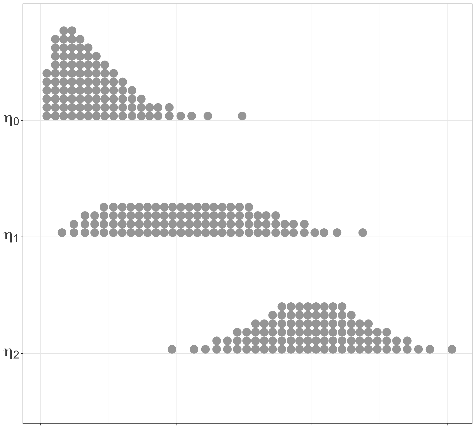
Fully adapted auxilary particle filter

Counter example from [JD, 2008]

M_0(x_0) = \begin{cases} \frac{1}{2}, & x_0 = 0\\ \frac{1}{2}, & x_0 = 1\\ \end{cases}

M_1(x_0, x_1) = \begin{cases} 1-\delta, & x_1 = x_0\\ \delta, & x_1 = 1-x_0\\ \end{cases}

Counter example from [JD, 2008]

G_t(x_t) = \begin{cases} 1-\epsilon, & x_t = y_t\\ \epsilon, & x_t = 1- y_t,\\ \end{cases}, \quad t \in \{0,1\} with fixed observations y_t.

Take y_0 = 0 and y_1 = 1 and

consider a test function \varphi(x_1) = x_1

Example: Binary FA-APF

Example: Binary FA-APF

Example: Non-linear Student distribution

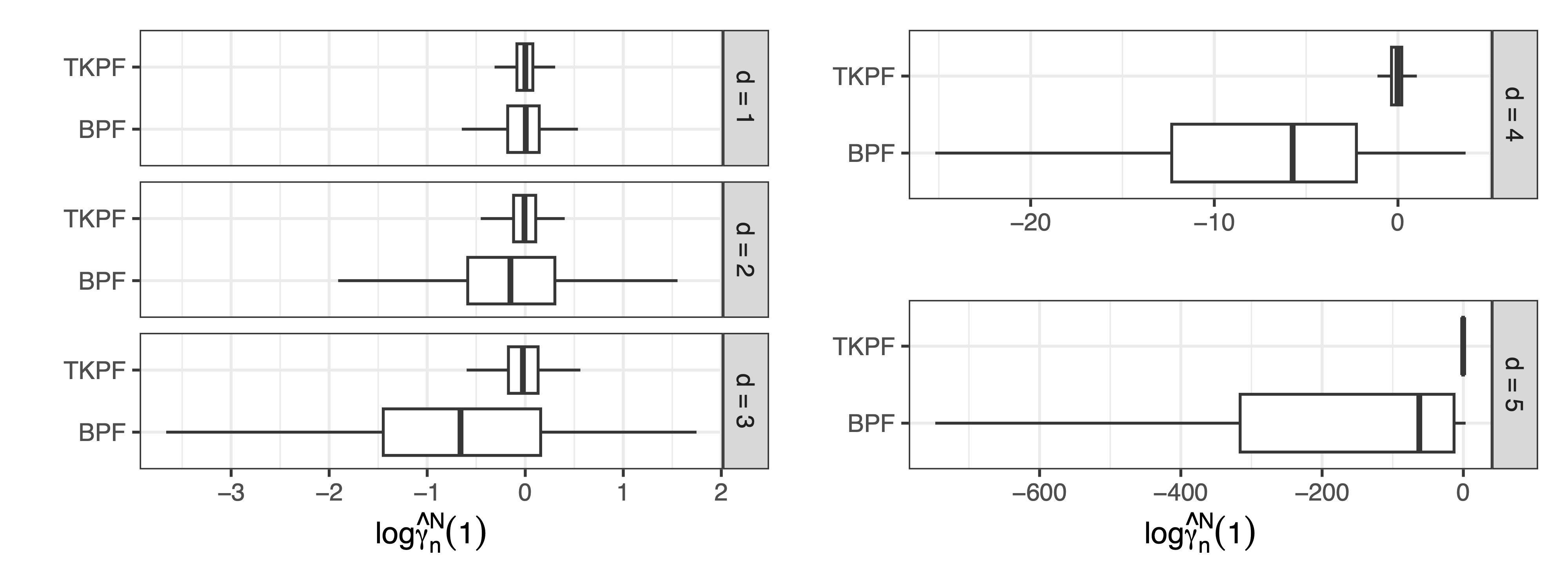
X_0\sim \mathcal{T}(\mu,\Sigma,\nu)

(X_p \mid X_{p-1}) \sim \mathcal{T}(f_p(X_{p-1}),\Sigma,\nu)~\text{for}~p\in[1:n]

Summary

• Knots are a tool for algorithm design

• Generalise Rao-Blackwellisation

• “Fix” the counter example in [J&D, 2008]

• Knots create an ordering of algorithms

• Not discussed

  • Terminal knots + normalising constants
  • Knotsets + optimality
  • Multiple applications of knots
  • SMC samplers

Thank you!

Appendix

Knots definition

Definition 1: Feynman–Kac knot

A knot \mathcal{K} is specified by a time t \in \mathbb{N}_{0}, and an ordered pair of composable Markov kernels R and K. We say \mathcal{K}=(t,R,K).

Note that R is a probability distribution when t=0.

Definition 2: Knot compatibility

Let \mathcal{M}=(M_{0:n},G_{0:n}) be a Feynman–Kac model.

A knot \mathcal{K}=(t,R,K) is compatible with \mathcal{M} if t < n and M_t = RK.

Knot operator

Definition 3: Knot operator

For knot \mathcal{K} = (t,R,K) and model \mathcal{M} = (M_{0:n},G_{0:n}),

the operation \mathcal{K} \ast \mathcal{M} = (M_{0:n}^\ast,G_{0:n}^\ast) where M_{t}^\ast = R, \quad G_t^\ast = K(G_t), \quad M_{t+1}^\ast = K^{G_t} M_{t+1}, with

• K^{G_t}(y_t, \mathrm{d} x_t) = \frac{K(y_t, \mathrm{d} x_t)G_t(x_t)}{K(G_t)(y_t)}

• M_{p}^\ast = M_{p} for p \notin \{t,t+1\}

• G_{p}^\ast = G_{p} for p \neq t

Effect of a knot

If \mathcal{M}^\ast = \mathcal{K}\ast \mathcal{M} where \mathcal{K}= (t,R,K) then

1. \gamma_n^\ast(\varphi) = \gamma_n(\varphi)

2. \gamma_t^\ast = \hat\gamma_{t-1} R

3. Q_{t,n}^\ast = K Q_{t,n}

Variance reduction

Theorem 1: Variance reduction from a knot

Consider models \mathcal{M} and {\mathcal{M}^\ast = \mathcal{K} \ast \mathcal{M}} for some knot \mathcal{K}. Let \mathcal{M} and \mathcal{M}^\ast have terminal measures \gamma_n and \gamma_n^\ast and asymptotic variance maps \sigma^2 and \sigma_\ast^2 respectively. If \varphi \in \mathcal{F}(\mathcal{M}) then the measures are equivalent \gamma_n(\varphi) = \gamma^\ast_n(\varphi) and the variances satisfy {\sigma_\ast^2(\varphi) \leq \sigma^2(\varphi)}.

Partial ordering and variance

Definition 4: A partial ordering

Consider two Feynman–Kac models, \mathcal{M},\mathcal{M}^\ast\in\mathscr{M}_n.

We say that {\mathcal{M}^\ast \preccurlyeq \mathcal{M}} if there exists a sequence of knots \mathcal{K}_1, \mathcal{K}_2,\ldots, \mathcal{K}_m such that \mathcal{M}^\ast = \mathcal{K}_m\ast\cdots\ast \mathcal{K}_1\ast\mathcal{M} for some m \in \mathbb{N}_{1}.

Theorem 2: Variance ordering

If {\mathcal{M}^\ast \preccurlyeq \mathcal{M}} then \sigma_\ast^2(\varphi) \leq \sigma^2(\varphi) for all \varphi where \sigma^2(\varphi) is finite.

Knotsets

Knotsets

Definition 5: Knotset

A knotset \mathcal{K}=(R_{0:n-1},K_{0:n-1}) is specified by n ordered pairs of composable kernels R_p and K_p. Note that for p=0, R_0 is a probability distribution.

Definition 6: Knotset compatibility

A knotset \mathcal{K}=(R_{0:n-1},K_{0:n-1}) is compatible with a Feynman–Kac

model \mathcal{M}=(M_{0:n},G_{0:n}) if M_p = R_p K_p for all p\in[0\,{:}\,n-1].

Knotsets operator

Definition 7: Knotset operator

For knotset \mathcal{K}= (R_{0:n-1},K_{0:n-1}) and model \mathcal{M}= (M_{0:n},G_{0:n}),

the operation \mathcal{K}\ast \mathcal{M}= (M_{0:n}^\ast,G_{0:n}^\ast) where \begin{alignat*}{3} M_0^\ast &= R_0, &\quad G_0^\ast &= K_0(G_0), & & \\ M_{p}^\ast &= K_{p-1}^\prime R_p, &\quad G_p^\ast &= K_p(G_p), & &\quad p \in [1\,{:}\,n-1] \\ M_{n}^\ast &= K_{n-1}^\prime M_{n}, &\quad G_n^\ast &= G_n & \end{alignat*} where K_p^\prime(y_p, \mathrm{d}x_p) = \frac{K_p(y_p, \mathrm{d}x_p)G_p(x_p)}{K_p(G_p)(y_p)} for p \in [0\,{:}\,n-1].

References

Dau, Hai-Dang, and Nicolas Chopin. 2022. “Waste-Free Sequential Monte Carlo.” Journal of the Royal Statistical Society Series B: Statistical Methodology 84 (1): 114–48.
Johansen, Adam M, and Arnaud Doucet. 2008. “A Note on Auxiliary Particle Filters.” Statistics & Probability Letters 78 (12): 1498–1504.